How to use this guide
Business statistics helps turn records into useful summaries and evidence. Logic helps you reason through statements, patterns and constraints without jumping to conclusions.
This guide follows the supplied MGU syllabus for MG1CCRBBA102. Topics marked “theory only” remain conceptual in this guide; the syllabus does not prescribe numerical problems for those items. No suggested question is claimed to be an actual or guaranteed MGU question.
Learning outcomes in plain language
- Recognise statistical ideas suited to a business scenario.
- Organise data and reason clearly.
- Apply statistical treatment to business data.
- Evaluate and interpret data with suitable techniques.
- Explain trends using appropriate statistical models.
Course map, priorities and assessment
→ CENTRE + SPREAD → SHAPE (SKEWNESS / KURTOSIS)
→ TWO VARIABLES → COVARIANCE / CORRELATION → REGRESSION & TREND
UNCERTAINTY → PROBABILITY RULES → DISTRIBUTION MODELS (THEORY)
CLAIM / PATTERN → LOGICAL REASONING & APTITUDE PROBLEMS
MUST MASTER: mean/median/mode, dispersion and CV; interpret skewness/kurtosis; correlation and regression; probability rules; aptitude and logic problem-solving; the two Excel assignments.
IMPORTANT: frequency tables and graphs, weighted mean, covariance, Spearman ranks, regression coefficients and business applications.
QUICK-SCORE: definitions, distinctions, distribution characteristics (theory only), logic terms and formula interpretation.
Priorities follow the course outcomes, ESE structure and assignment requirements—not invented topic-wise marks.
Official ESE pattern
| Question type | Choice | Marks |
|---|---|---|
| 2-mark short answers from last two units | Answer 5 of 8 | 10 |
| 5-mark short essays (problem and theory) | Answer 4 of 6 | 20 |
| 20-mark essays (problem and case study) | Answer 2 of 4 | 40 |
| Total | 70 |
CCA is 30 marks. The syllabus lists 4 learning hours in the lecture column, but does not clearly state total course hours in the extracted table; no total is assumed here.
Organise, summarise and describe data
You will learn: classification, tabulation, frequency distributions, diagrams/graphs, measures of centre and spread, skewness and kurtosis.
Why it matters: a manager needs a clear summary before comparing sales, costs, customer responses or performance.
Classifying and tabulating data
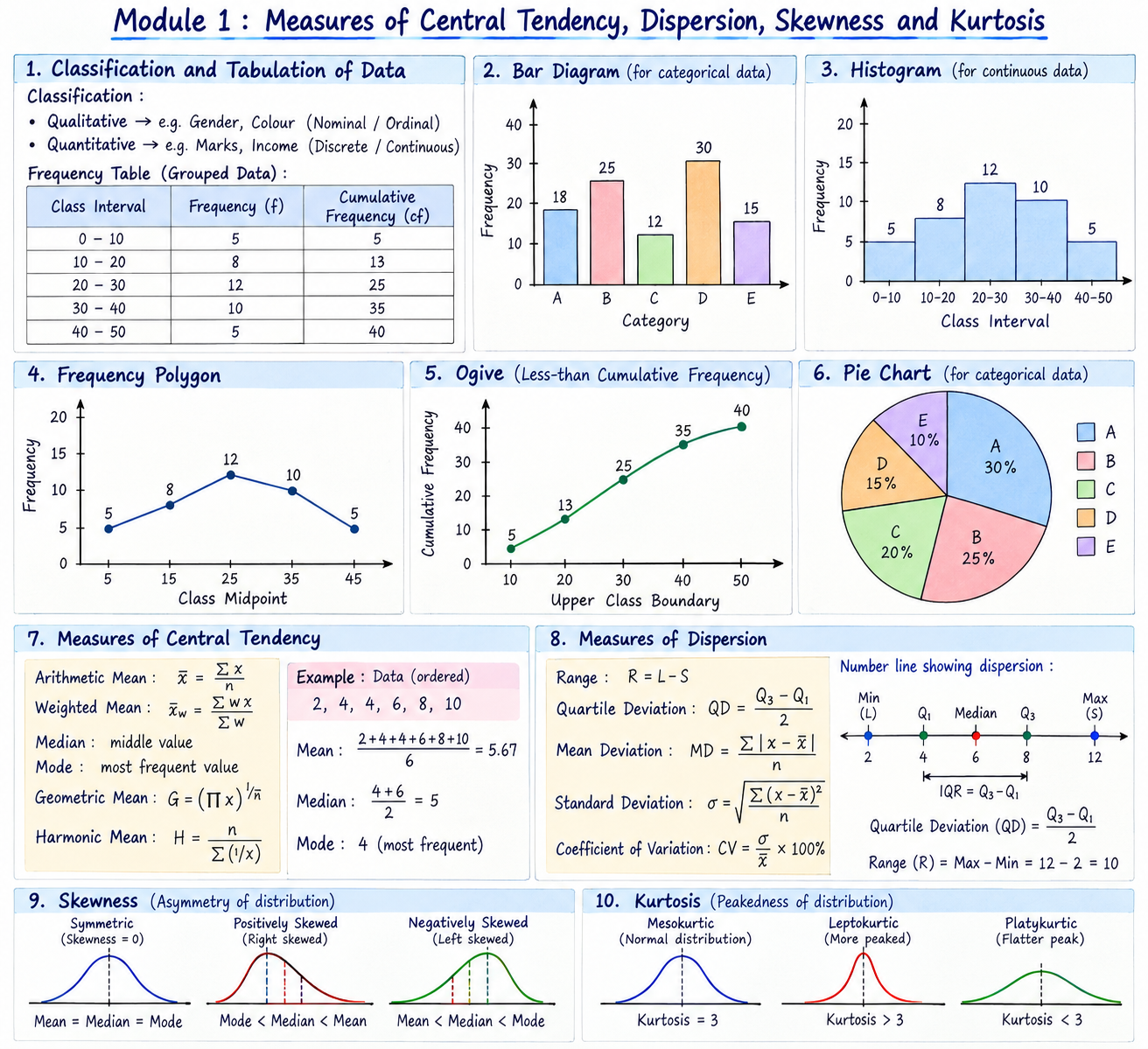
Classification groups observations by shared features. A frequency distribution lists values or intervals and how many observations fall in each. A table should have a clear title, labels, units and totals.
Bar charts compare categories; histograms show grouped numerical distributions with touching bars; line graphs are useful for ordered time data. Label axes and avoid distorted scales.
Measures of central tendency
A measure of central tendency gives a typical or central value.
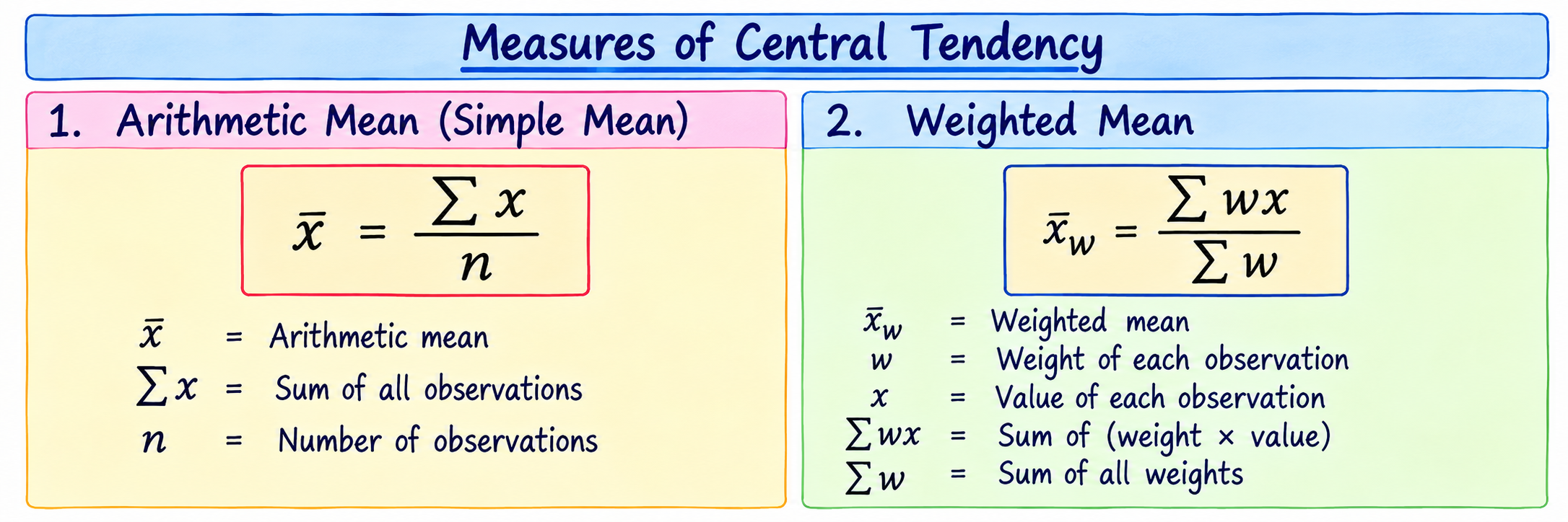
For the weighted mean, x is a value and w its weight (e.g. units sold or credit weight). The denominator is total weight.
Median: order values and take the middle (or average the two middle values). Mode: most frequent value. Geometric mean (GM), theory only: the nth root of the product of n positive values; describes multiplicative average growth. Harmonic mean (HM), theory only: n divided by the sum of reciprocals; useful conceptually for averaging rates over equal units. The syllabus labels GM/HM theory only.
Measures of dispersion
Dispersion describes how spread out observations are. Two product lines can have equal average sales but different stability.
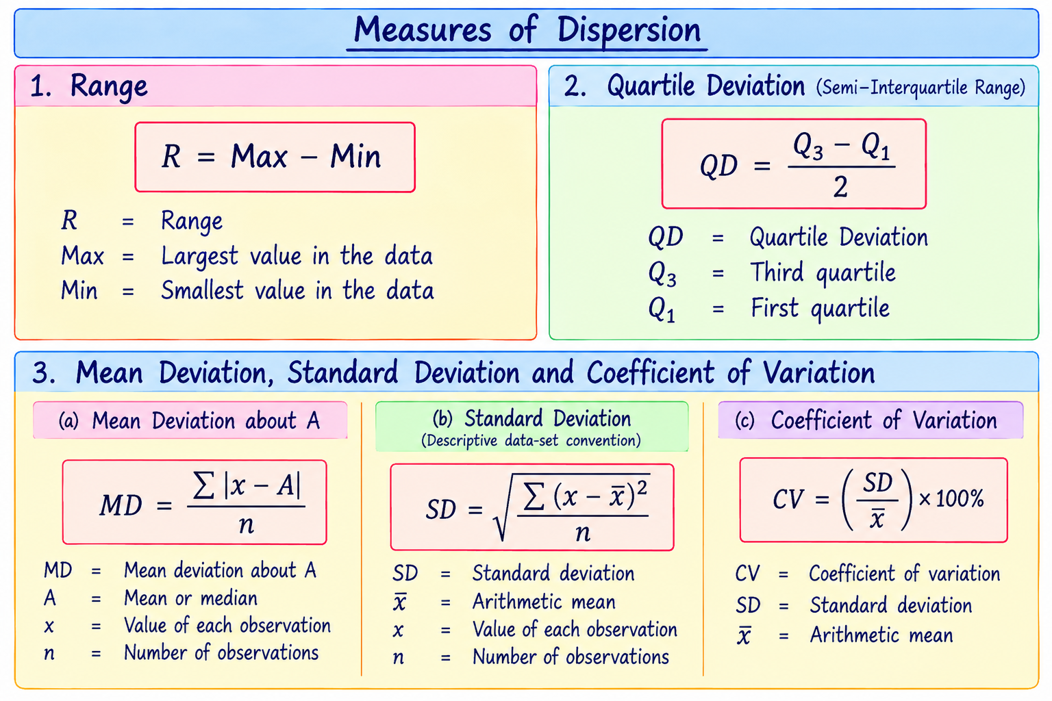
Range uses only the extremes; quartile deviation describes the middle half; mean deviation averages absolute distances; SD measures typical spread around the mean; CV compares spread relative to the mean.
State the convention for quartiles and SD used in your class when it affects the answer.
Skewness and kurtosis
Skewness describes asymmetry. A longer right tail is positive skew; a longer left tail is negative skew. In a roughly symmetric distribution, mean and median are often close. Kurtosis describes aspects of tail/peak shape relative to a reference distribution; software conventions may report kurtosis or excess kurtosis, so read the function’s definition.
Use a histogram to see shape. The mean, median and SD alone do not fully describe skewness or tail behaviour.
Module 1 recap
Key terms: frequency, class interval, weighted mean, median, mode, range, quartile, mean deviation, standard deviation, coefficient of variation, skewness, kurtosis.
Exam-focused: calculate descriptive measures; explain why dispersion matters; interpret a histogram; describe skewness/kurtosis and their business relevance.
Self-test: (1) Which centre resists extreme values? (2) What does CV compare? (3) What shape has a longer right tail? (4) Why is a weighted mean useful for average selling price?
Describe relationships and estimate trends
You will learn: covariance, scatter diagrams, correlation types, Pearson and Spearman coefficients, probable error (theory only), and regression lines/equations/coefficients.
Why it matters: businesses often ask whether two quantities vary together and how one may be estimated from another.
Correlation, scatter and covariance
Correlation describes direction and strength of association. Plot paired observations (x,y) on a scatter diagram first. An upward pattern is positive; downward is negative; a diffuse pattern suggests weak linear association.
Covariance measures whether paired values tend to deviate from their means in the same direction (positive) or opposite directions (negative). Its magnitude depends on measurement units; correlation standardises this relationship.
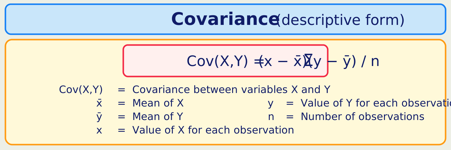
For sample covariance, some courses use denominator n−1. Follow the convention specified in the problem or taught in class.
Karl Pearson and Spearman rank correlation
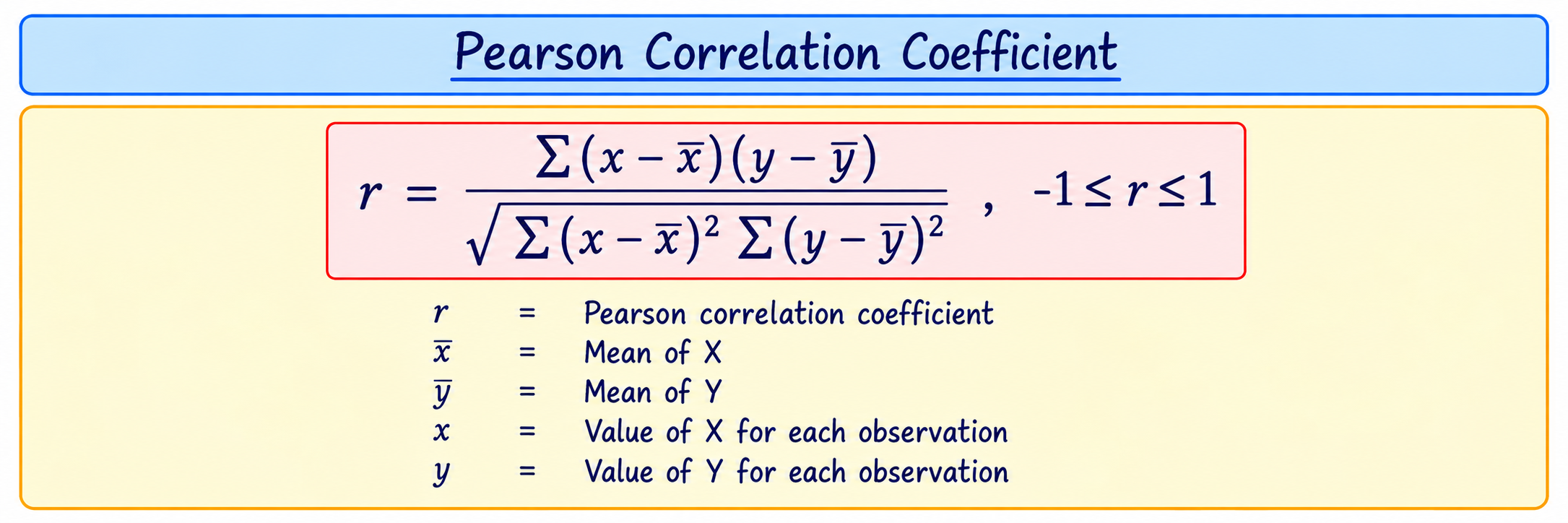
The sign gives direction; magnitude nearer 1 means stronger linear association. Correlation does not prove causation and r near zero does not rule out a curved relationship.
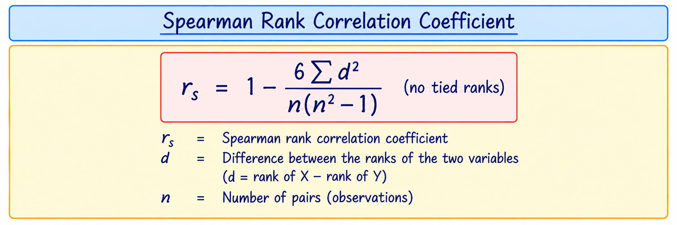
d is the difference between paired ranks. Rank each variable consistently; use the tie method prescribed when ties occur.
Probable error (theory only): a historical measure used in discussing the reliability of a sample correlation. The syllabus specifies theory only; learn its definition and interpretation from the class/reference convention, and do not treat it as a substitute for a modern test or causal evidence.
Regression
Regression describes a fitted relationship for estimating one variable from another. Correlation summarises association symmetrically; regression chooses a response variable and predictor, so x-on-y and y-on-x are different lines.
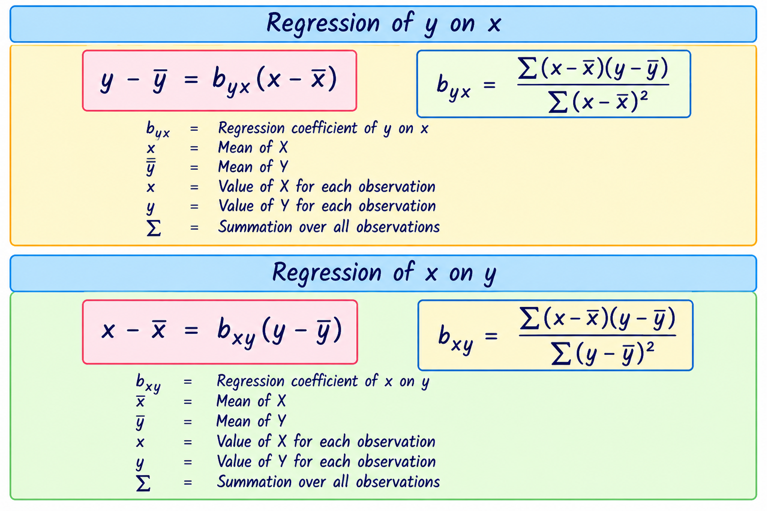
The slope is the estimated change in response per one-unit predictor change. Choose y-on-x to estimate y when x is known. A regression line is an estimate, not a guarantee; avoid predictions far outside observed values.
Module 2 recap
Key terms: paired data, scatter diagram, covariance, correlation, Pearson coefficient, rank, Spearman coefficient, probable error, regression, slope, prediction.
Exam-focused: interpret a scatter; calculate Pearson/Spearman; explain probable error in theory; distinguish correlation from regression; obtain/use regression equations and coefficients.
Self-test: (1) What does r=−0.8 suggest? (2) Why rank for Spearman? (3) Which regression line estimates y from x? (4) Can correlation establish cause?
Reason about uncertainty
You will learn: classical probability, addition/multiplication rules and theory of binomial, Poisson and normal distributions.
Why it matters: business decisions are made with uncertain demand, delays and outcomes. Probability makes uncertainty explicit.
Basic probability and classical definition
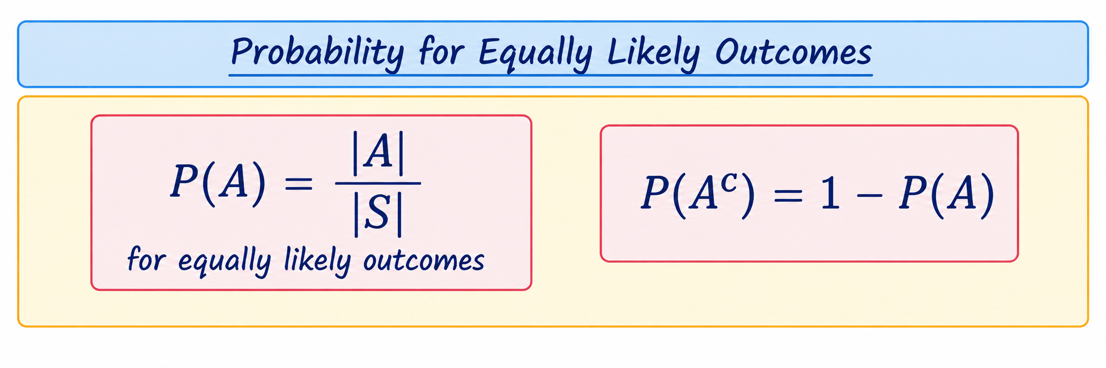
For equally likely outcomes, probability of event A is favourable outcomes divided by total outcomes. Probability is between 0 and 1; 0 means impossible in the model, 1 certain.
Addition and multiplication rules
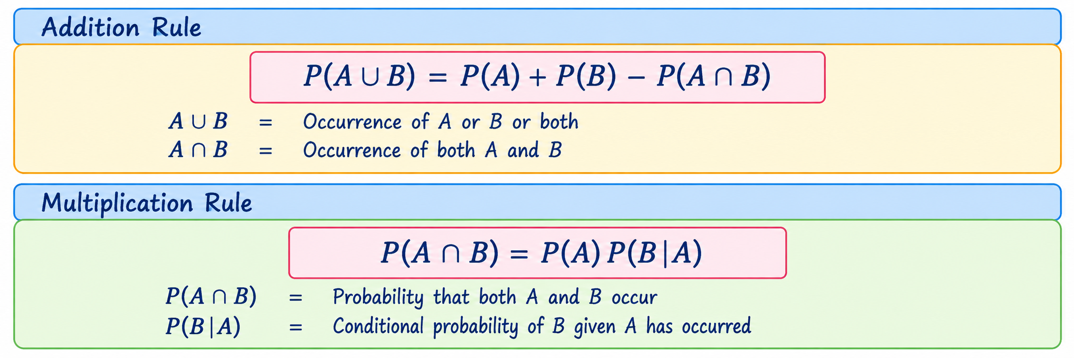
If A and B are mutually exclusive, P(A∩B)=0, so add probabilities directly.
For independent events this becomes P(A∩B)=P(A)P(B). Do not assume independence unless the situation states it or it is justified.
Binomial, Poisson and normal distributions — theory only
The syllabus explicitly lists these distributions as theory only. Be prepared to explain what each models, its characteristic conditions and general shape; this guide does not treat their numerical calculations as prescribed examination scope.
| Distribution | What it models | Key recognition |
|---|---|---|
| Binomial | Number of successes in a fixed number of trials | Two outcomes per trial; same success probability; independent trials |
| Poisson | Count of events in a fixed interval under a stated average rate model | Nonnegative integer count; parameter is average rate λ |
| Normal | Continuous, symmetric, bell-shaped model | Described by mean and standard deviation; observations cluster around mean |
Compare: binomial has a fixed number of attempts; Poisson focuses on counts per interval; normal describes a continuous measurement. Avoid choosing a model from its name alone—check the scenario assumptions.
Module 3 recap
Key terms: experiment, outcome, event, equally likely, complement, union, intersection, mutually exclusive, independent, distribution.
Exam-focused: compute basic classical probabilities; apply addition/multiplication rules; explain binomial/Poisson/normal characteristics in theory.
Self-test: (1) When may favourable/total be used? (2) Why subtract P(A∩B) in the addition rule? (3) What makes two events independent? (4) Which named model describes a fixed number of success/failure trials?
Aptitude patterns and reasoning
You will learn: number series, coding-decoding, odd-one-out series, direction sense, linear/circular seating, blood relations, arithmetic/geometric progressions, inductive and deductive reasoning.
Why it matters: these activities train pattern recognition and structured reasoning used in business decisions and competitive aptitude tests.
Number series and odd one out
Look for a consistent rule between terms: constant difference, multiplication, alternating operations, squares/cubes or two interleaved sequences. For odd-one-out, compare a stated feature across every item and identify the one that breaks the common rule.
Coding and decoding
Compare letter or number positions, shifts, reversals, alternating rules and repeated patterns. Write the mapping explicitly before applying it. Do not infer a code from one example if another example contradicts it.
Direction sense
Draw a small compass and track each turn and distance. A right turn changes facing clockwise; a left turn changes it anticlockwise. Separate final facing direction from displacement (where the person ends relative to the start).
Seating arrangements
For a linear arrangement, draw positions in a row. For a circular arrangement, mark seats around a circle and use a consistent viewpoint; facing inward/outward changes left-right interpretation. Add one constraint at a time and cross out contradictions.
Blood relations
Translate each phrase into a family link and draw a small tree. Keep speaker perspective clear: “my mother’s brother” and “her brother” may refer to different people depending on who is speaking.
Arithmetic and geometric progressions
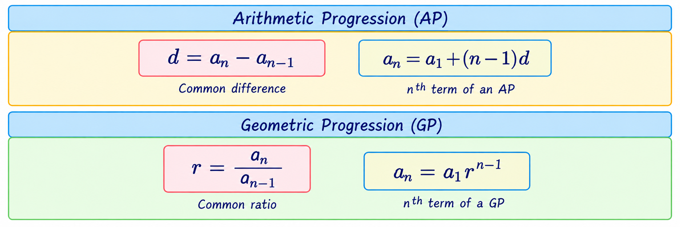
An arithmetic progression (AP) adds the same number each step. A geometric progression (GP) multiplies by the same ratio. Check the pattern and whether the question asks for a term, sum or rule.
Inductive and deductive reasoning
Inductive reasoning uses observations or examples to suggest a general pattern; the conclusion is plausible but may not be certain. Deductive reasoning applies general rules/premises to reach a conclusion that must follow if those premises are true.
Module 4 recap
Key terms: pattern, sequence, code, displacement, orientation, constraint, linear arrangement, circular arrangement, induction, deduction.
Exam-focused: solve aptitude questions systematically, show a diagram/table where useful, distinguish inductive from deductive reasoning, and apply AP/GP rules.
Self-test: (1) What is the AP common difference in 4,7,10? (2) What is the GP ratio in 2,6,18? (3) Why draw direction moves? (4) Is a pattern inferred from several examples deductive or inductive?
Excel assignments and project preparation
The syllabus describes two assignments. Use the exact requirements and mark allocation given by your lecturer.
Assignment A · Group (5 marks)
Use Excel and course statistics to analyse real-world primary or secondary data and interpret results. The syllabus gives sales data or environmental indicators as examples and suggests exploring correlation/regression for expenditure and income data from 50 students.
- State the question and identify data source, variables, units and sample size.
- Keep raw data in a clearly labelled table; note missing values or coding.
- Calculate suitable summaries (e.g. mean, median, mode, SD, range) where relevant.
- For paired variables, create a scatter diagram and calculate correlation/regression if suitable.
- Explain the output in context; state limitations and avoid causal claims unless design supports them.
- Present a brief report with method, results, tables/graphs and conclusion.
Assignment B · Individual (4 marks)
Choose a real-life numerical data set, calculate basic statistics, identify skewness/kurtosis, and visualise it with a histogram and normal curve overlay.
- Describe the data source and variable, with units and number of observations.
- Calculate mean, median, mode and SD.
- Calculate skewness/kurtosis using the convention required by class/software; label whether reported kurtosis is excess or raw.
- Create a labelled histogram; overlay the normal curve using a compatible scale (density scale or frequency-scaled curve).
- Describe whether the observed shape is symmetric/skewed and how it differs from the reference curve.
Do not claim the data are normal only because a curve was drawn; treat the overlay as a visual comparison.
Formula sheet and answer-writing
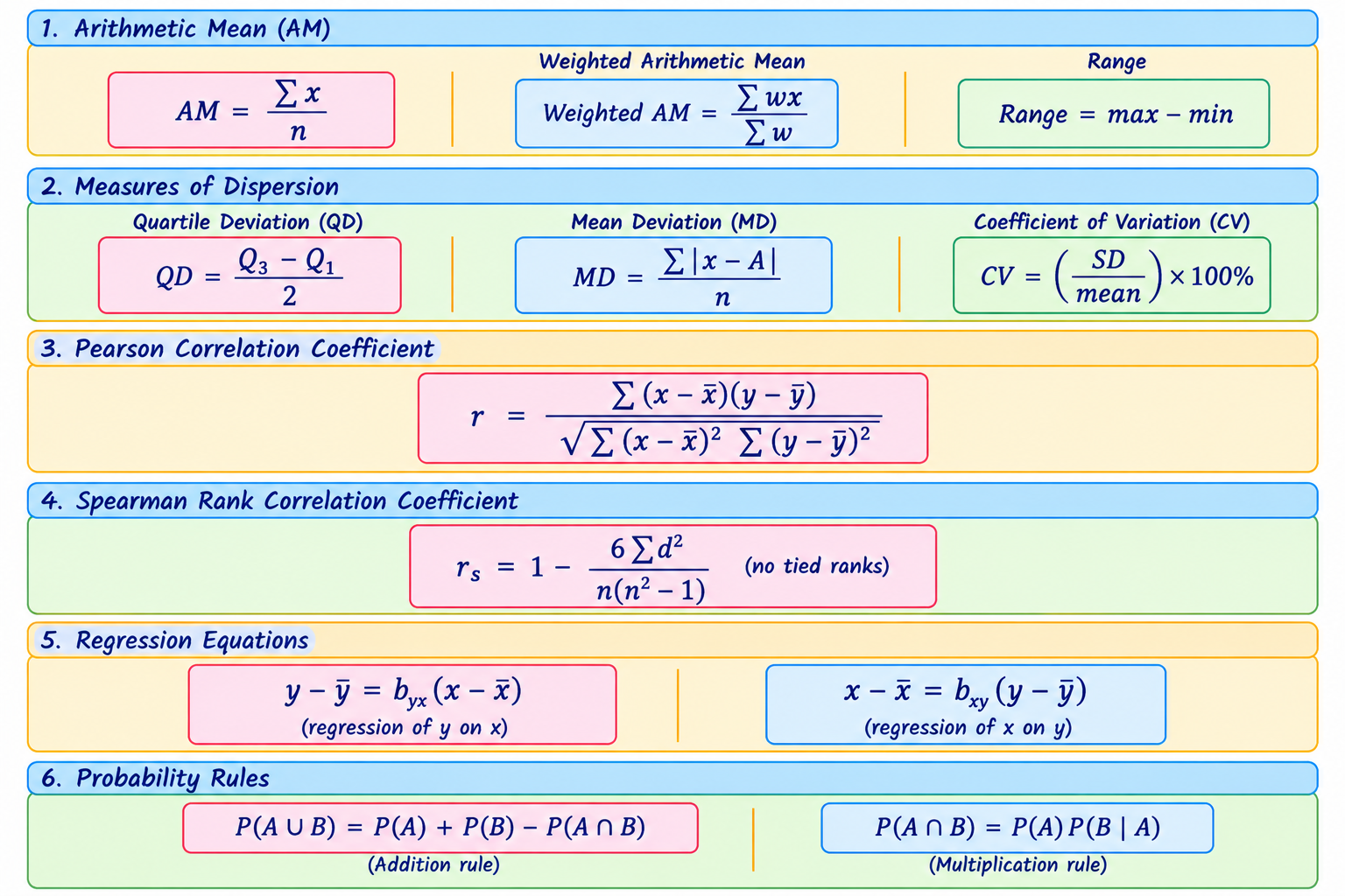
For a numerical answer show: given → required → formula → substitution → calculation → result → interpretation. For a case study, include the business question, data, method, result, limitation and recommendation supported by the evidence.