Introduction to Statistical Modelling

1.1 Random variables: discrete and continuous

A random variable assigns a number to each outcome of a random experiment. It is usually written X. The number need not itself be uncertain after the experiment; it is uncertain before the outcome is known.

Discrete means countable separate values; continuous means values over a continuum/interval. A measured continuous quantity is often rounded in practice, but its model can still be continuous.

1.2 PMF, PDF and CDF

A probability mass function (PMF) gives the probability of each value of a discrete random variable. A probability density function (PDF) describes density for a continuous variable; probabilities are areas, not heights. The cumulative distribution function (CDF) gives the probability that X is at most x.

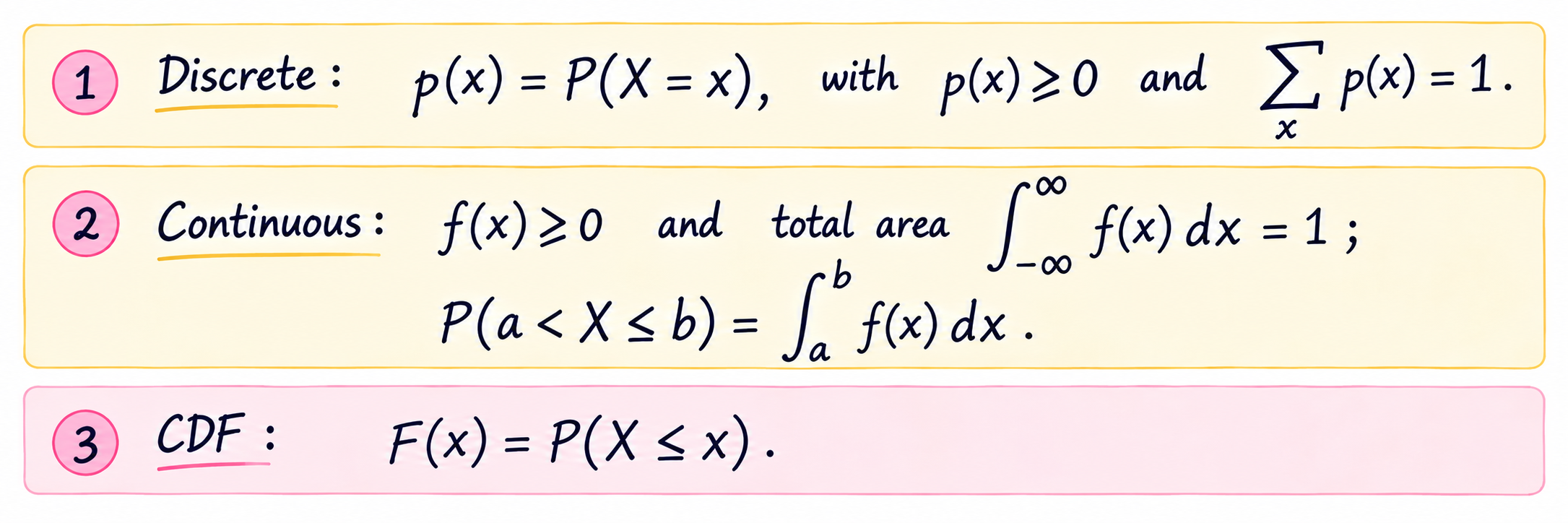
For a discrete X, add PMF values up to x. For a continuous X, integrate the PDF up to x. A CDF never decreases, approaches 0 far to the left and 1 far to the right, and probability over an interval is obtained from the difference of CDF values.

1.3 Functions and transformations (univariate)

If X is random and Y=g(X), then Y is also random. A transformation changes the value assigned to each outcome. For a discrete variable, list possible X values, calculate g(x), and combine probabilities when different x values produce the same y.

For a continuous variable, one basic method is to find the CDF of Y from Fᵧ(y)=P(g(X)≤y), then differentiate when the resulting CDF has a density.

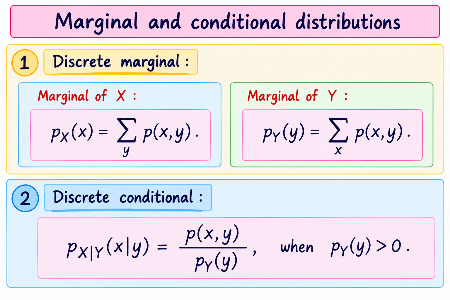
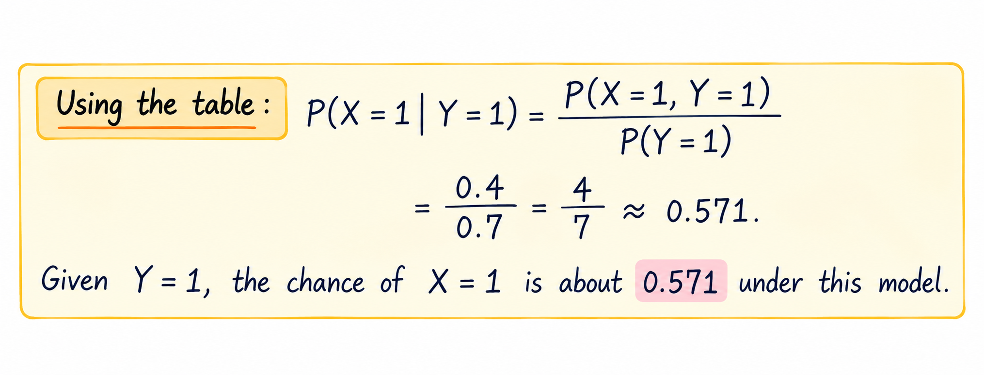
For continuous variables, replace sums with integrals and divide joint density by the relevant marginal density.

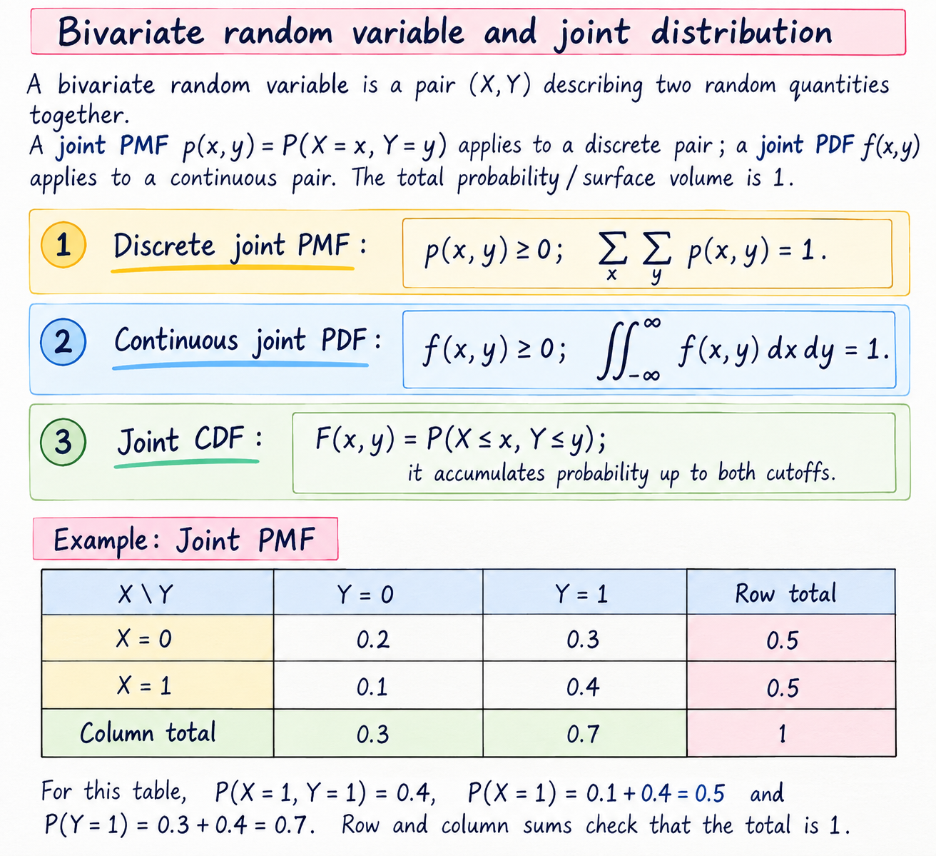
X and Y are independent if knowing one does not change the distribution of the other. For discrete variables, check p(x,y)=pX(x)pY(y) for all pairs. In the table, p(1,1)=0.4 but pX(1)pY(1)=0.5×0.7=0.35, so X and Y are not independent.

2.1 Mathematical expectation

Expectation is the long-run probability-weighted average of a random variable. It is not necessarily a value the variable can actually take.

Each possible value is weighted by its probability or density; for a valid finite expectation, the required sum/integral must exist.

Linearity: E(aX+b)=aE(X)+b. For sums, E(X+Y)=E(X)+E(Y), even without independence, provided expectations exist.

2.2 AM, GM, HM, mean deviation and variance in terms of expectation

Variance is expected squared distance from the mean. Standard deviation is its square root, returning to the original measurement units.

For a random variable, the probability-weighted arithmetic mean is E(X). For positive values, geometric and harmonic means can be expressed using logs and reciprocal values: GM=exp(E[ln X]) and HM=1/E(1/X), where the expectations exist. For a finite equally weighted data set these reduce to the familiar formulas from Semester 1. The syllabus asks for simple problems.

Useful properties: Var(aX+b)=a²Var(X); adding a constant shifts the mean but not the spread. If X and Y are independent, Var(X+Y)=Var(X)+Var(Y). Do not apply the last equality without the independence condition (or other appropriate covariance information).

2.3 Moment-generating and characteristic functions

A generating function turns distribution information into a function. Differentiating a moment-generating function at zero gives moments when it exists near zero.

For independent variables, the MGF of a sum is the product of their MGFs when the relevant MGFs exist. This can simplify sums and help identify distributions.

The characteristic function exists for every probability distribution and is complex-valued in general. It also encodes distribution information. At this syllabus level focus on definition, properties covered in class and simple problems, not advanced inversion theory.

3.1 Discrete uniform, Bernoulli and binomial

Discrete uniform: each of the n listed outcomes has probability 1/n. For a fair six-sided die, P(X=x)=1/6 for x=1,…,6.

Bernoulli: one trial with two outcomes, coded success (1) with probability p and failure (0) with probability 1−p. Mean p; variance p(1−p).

Binomial: counts successes in n independent Bernoulli trials with the same success probability p.

C(n,k) counts ways to place k successes among n trials. The factors represent k successes and n−k failures. Check fixed n, two outcomes per trial, constant p and independence.

3.2 Poisson and geometric distributions

Poisson: models a count of occurrences in a specified interval when an average rate λ is appropriate. Support is 0,1,2,…

Geometric: number of independent trials up to and including the first success, with constant success chance p. This guide uses support 1,2,…; state the convention because some texts count failures before success.

The last equality is the lack-of-memory property: conditional on still waiting after m failures, the additional wait has the original geometric distribution.

3.3 Continuous uniform distribution

If X is equally spread across an interval [a,b], its density is constant there. Probability is interval length divided by total length.

3.4 Exponential and gamma distributions

Exponential: models a nonnegative waiting time with rate λ>0.

The exponential distribution has lack of memory: P(X>s+t | X>s)=P(X>t). Knowing that a wait has already lasted s does not change the model distribution of the additional wait.

Gamma: a continuous distribution on x>0 with shape α>0 and rate λ>0 in the rate parameterisation below. It generalises waiting-time models; when α=1 it is exponential with rate λ.

Γ(α) is the gamma function/normalising factor that makes total density area 1. If your class uses a scale parameter θ=1/λ, use the corresponding form and state which parameterisation you use.

3.5 Normal distribution and standard normal table

The normal distribution is a continuous, symmetric, bell-shaped model determined by mean μ and variance σ². Values near μ are more common; the curve’s total area is 1.

Standardisation measures how many standard deviations x lies above or below the mean. A standard normal table may give left-tail Φ(z)=P(Z≤z); always check the table heading.

For intervals, translate both endpoints to z-scores and use the table consistently: P(a<X<b)=Φ(zᵦ)−Φ(zₐ). Symmetry gives Φ(−z)=1−Φ(z).

Ten-plus practical record ideas

1. Create a discrete PMF table; check probabilities sum to 1; calculate its CDF.
2. Use a joint PMF table to obtain marginal distributions and verify totals.
3. Calculate a conditional distribution from a joint table; test independence.
4. Calculate E(X), E(X²), variance and standard deviation from a PMF.
5. Use a Bernoulli/binomial function or formula to calculate event probabilities.
6. Calculate Poisson probabilities for several k values and compare cumulative probability.
7. Calculate geometric probabilities and verify a finite partial sum is at most 1.
8. Use continuous uniform and exponential CDF formulas for interval/tail probabilities.
9. Standardise observations and use the software’s normal CDF/inverse functions; compare with a standard normal table.
10. Simulate repeated Bernoulli trials using a random-number function; compare empirical proportion with p.
11. Simulate binomial counts or waiting times and compare a frequency graph with theoretical probabilities.

Use the software available in your practical class. Function names differ; typical spreadsheet programs provide binomial, Poisson and normal distribution functions and random-number generation. Record the exact function and argument order used.

Practical/viva preparation

• What do PMF, PDF and CDF spreadsheet outputs represent?
• How do you check that a discrete distribution is valid?
• How do you obtain a marginal distribution from joint data?
• Which cell references change when a formula is copied? How can a reference be made absolute?
• Why does a simulation not exactly equal its theoretical probability in a finite number of trials?
• How can you compare observed and theoretical probabilities using a table or graph?
• How did you choose the distribution and its parameters in your practical record?

For each submitted record problem, include: objective, given data/parameters, formula or function, output, one verification, interpretation and conclusion.